Octagon Algorithm for Border Wheel Squares (Part VI)
The Eight Node Way - 5×5 Squares
The previous section Part IV introduced the Octagon E and F algorithm for the construction of 5×5 Wheel Squares. The main diagonal of the wheel structure was filled in in reverse order (12,11,13,15,14) in order to produce the new border squares. This section will depict the Wheel Border where the main diagonal is in regular order but the rows and columns of the wheel are constructed so that the difference (Δ) between each term is 3, 5 or 7 units. These Δ values are important in that they allow us to construct different wheel structures in the square as long as there are enough numbers in the complement table to construct a wheel.
If not, then there is a maximum number of wheel structures allowed for a particular order n. It will be shown that the number of wheel structures decreases as Δ increases. For instance, for n=5 when Δ = 3, 5 and 7 the number of consecutive border squares that can be constructed is 3, 2 and 1, respectively. By consecutive is meant that the starting number for the first three spokes is a,b,c where a, b and c are one unit apart. For instance, Wheels G, H and I can have the starting values of (1,2,3), (3,4,5) or (5,6,7), respectively.
A table for Δ values vs the order n can be found in Part VIII. When Δ values are greater than 7 for a 5th order square it is not possible to construct border squares due to an insufficient number of terms in the complement table. Thus, the maximum value that Δ can take is n + 2 for consecutive spoke numbers chosen from the complementary table. A total of six squares with the above Δ values will be shown below for the two different Octagonal algorithms.
To start, the wheel part of the square is first constructed using either of the three (Δ) values followed by the non wheel portion (i.e, non spokes) which uses either the Octagon G or H algorithm to fill in the empty cells. The method can be summarized as follows where regular means with a degree of separation (Δ) between numbers:
a) the main diagonal is first filled in with the numbers 11,12,13,14,15
b) the central column is filled in regular order starting at the topmost cell and moving to the bottom cell
c) the left diagonal is filled in regular order starting at the right bottom cell and moving to the leftmost top cell
d) the central row is filled in regular order starting at the leftmost cell and moving to the rightmost cell
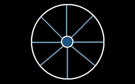
Thus, three wheels which can be produced using the wheel algorithm: Wheel G, Wheel H and Wheel I:
Wheel G
| 24 | |
1 | |
15 |
| 21 |
4 | 14 |
|
| 3 | 6 |
13 | 20 |
23 |
| 12 |
22 | 5 |
|
| 11 | |
25 | |
2 |
|
|
Wheel H
| 22 | |
3 | |
15 |
| 19 |
6 | 14 |
|
| 5 | 8 |
13 | 18 |
21 |
| 12 |
20 | 7 |
|
| 11 | |
23 | |
4 |
|
|
Wheel I
| 20 | |
5 | |
15 |
| 17 |
8 | 14 |
|
| 7 | 10 |
13 | 16 |
19 |
| 12 |
18 | 9 |
|
| 11 | |
21 | |
6 |
|
which uses the accompaning 5×5 complementary table as a guide to pick the 17 wheel spoke numbers and 8 of the non spoke numbers:
| 1 | 2 |
3 | 4 |
5 | 6 |
7 | 8 |
9 | 10 |
11 | 12 |
|
| 13 |
| 25 | 24 |
23 | 22 |
21 | 20 |
19 | 18 |
17 | 16 |
15 | 14 |
|
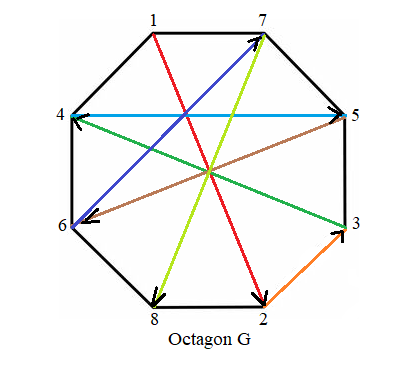
To fill in the remainder of the numbers a new algorithm, Octagon G, is used starting with the initial node at the top left of the octagon:
We start by adding the lowest spoke number on the complementary table to position (1,0), i.e., position (row, column), on the square. For example, in Wheel G, the first non spoke number, 7, goes into the cell corresponding to node 1. Using Octagon G one follows the arrows and deposits a number into the appropriate white cell of the square to generate the three squares:
Border 5(03)g
| 24 | 7 |
1 | 18 |
15 |
| 10 | 21 |
4 | 14 |
16 |
| 3 | 6 |
13 | 20 |
23 |
| 17 | 12 |
22 | 5 |
9 |
| 11 | 19 |
25 | 8 |
2 |
|
|
Border 5(13)g
| 22 | 1 |
3 | 24 |
15 |
| 10 | 19 |
6 | 14 |
16 |
| 5 | 8 |
13 | 18 |
21 |
| 17 | 12 |
20 | 7 |
9 |
| 11 | 25 |
23 | 2 |
4 |
|
|
Border 5(23)g
| 20 | 1 |
5 | 24 |
15 |
| 4 | 17 |
8 | 14 |
22 |
| 7 | 10 |
13 | 16 |
19 |
| 23 | 12 |
18 | 9 |
3 |
| 11 | 25 |
21 | 2 |
6 |
|
where the numbering, for example, 5(03)g correponds to n=5, 0 is the wheel type, 3 is the Δ and g is the algorithm used in this case Octagon G.
When the value of Δ = 5 or 7, the following three squares are constructible:
Border 5(05)g
| 24 | 4 |
1 | 21 |
15 |
| 10 | 19 |
6 | 14 |
16 |
| 3 | 8 |
13 | 18 |
23 |
| 17 | 12 |
20 | 7 |
9 |
| 11 | 22 |
25 | 5 |
2 |
|
|
Border 5(15)g
| 22 | 1 |
3 | 24 |
15 |
| 8 | 17 |
8 | 14 |
18 |
| 5 | 10 |
13 | 16 |
21 |
| 17 | 12 |
18 | 9 |
7 |
| 11 | 25 |
23 | 2 |
4 |
|
|
Border 5(07)g
| 24 | 4 |
1 | 21 |
15 |
| 7 | 17 |
8 | 14 |
19 |
| 3 | 10 |
13 | 16 |
23 |
| 20 | 12 |
18 | 9 |
6 |
| 11 | 22 |
25 | 5 |
2 |
|
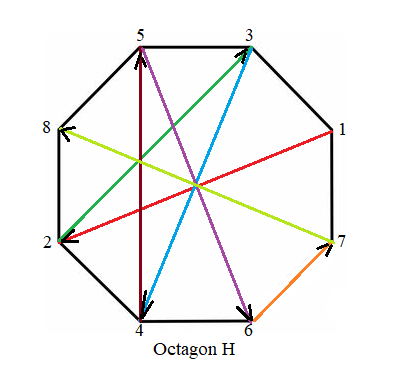
In the second algorithm, Octagon H with node 1 located at the middle right of the octagon, is employed to construct the second series of border 5×5 squares.
When Δ has a value of three the following consecutive squares can be constructed:
Border 5(03)h
| 24 | 16 |
1 | 9 |
15 |
| 19 | 21 |
4 | 14 |
17 |
| 3 | 6 |
13 | 20 |
23 |
| 8 | 12 |
22 | 5 |
18 |
| 11 | 10 |
25 | 17 |
2 |
|
|
Border 5(13)h
| 22 | 16 |
3 | 9 |
15 |
| 25 | 19 |
6 | 14 |
1 |
| 5 | 8 |
13 | 18 |
21 |
| 2 | 12 |
20 | 7 |
24 |
| 11 | 10 |
23 | 17 |
4 |
|
|
Border 5(23)h
| 20 | 22 |
5 | 3 |
15 |
| 25 | 17 |
8 | 14 |
1 |
| 7 | 10 |
13 | 16 |
19 |
| 2 | 12 |
18 | 9 |
24 |
| 11 | 4 |
21 | 23 |
6 |
|
|
Border 5(23)h
| 20 | 22 |
5 | 3 |
15 |
| 25 | 17 |
8 | 14 |
1 |
| 7 | 10 |
13 | 16 |
19 |
| 2 | 12 |
18 | 9 |
24 |
| 11 | 4 |
21 | 23 |
6 |
|
When the value of Δ = 5 or 7, the following three squares are constructible:
Border 5(05)h
| 24 | 16 |
1 | 9 |
15 |
| 22 | 19 |
6 | 14 |
4 |
| 3 | 8 |
13 | 18 |
23 |
| 5 | 12 |
20 | 7 |
21 |
| 11 | 10 |
25 | 17 |
2 |
|
|
Border 5(15)h
| 22 | 16 |
3 | 9 |
15 |
| 25 | 17 |
8 | 14 |
1 |
| 5 | 10 |
13 | 16 |
21 |
| 2 | 12 |
18 | 9 |
24 |
| 11 | 10 |
23 | 17 |
4 |
|
|
Border 5(07)h
| 24 | 19 |
1 | 6 |
15 |
| 22 | 17 |
8 | 14 |
4 |
| 3 | 10 |
13 | 16 |
23 |
| 5 | 12 |
18 | 9 |
21 |
| 11 | 7 |
25 | 20 |
2 |
|
In addition, Border 5(23)h is the way these border squares are normally depicted to show the magic properties of the internal and outer squares. The upshot is that both these algorithms along with the reversed wheel algorithm produce border squares, where the inner 3×3 squares have magic sums of 39 and the outer 5×5 squares have magic sums of 65.
This completes the Octagon G and H method for 5×5 squares.
Go to 7×7 Squares. Go back to homepage.
Copyright © 2022 by Eddie N Gutierrez. E-Mail: enaguti1949@gmail.com