The Reverse Wheel Method (XII) - A Switcheroo
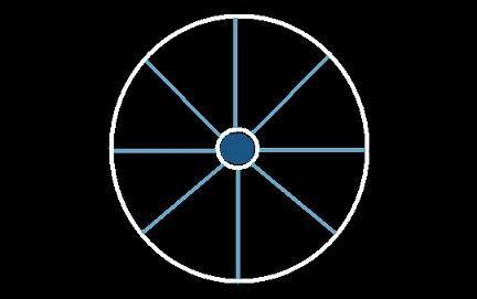
A Discussion of the Method
This method follows the modified wheel algorithm except that the complementary table from which the numbers are chosen
is the reverse of the normal complementary table. Reversal produces:
| 13 | 12 |
11 | 10 |
9 | 8 |
7 | 6 |
5 | 4 |
3 | 2 |
|
| 1 |
| 14 | 15 |
16 | 17 |
18 | 19 |
20 | 21 |
22 | 23 |
24 | 25 |
|
In addition the new squares formed are not magic but must be modified to convert them into magic squares. The square is filled as in the modified wheel fashion
and the wheel spoke numbers are picked from a complementary table, e.g., the 5x5 above in the reverse fashion.
Moreover, it must be stated here that the magic sum has been modified from the known equation
S = ½(n3 + n) to
the general equation as was shown in:
S = ½(n3 ± an)
which takes into account these new squares. The variable a, an odd number, is equal to 1,3,5,7 or ... and may take on + or -
values. For example when a = 1 the normal magic sum S is implied.
When a takes on different odd values S gives the magic sum of a modified magic square.
It will be shown that the addition or subtraction of n2 to some of the cells in
the square gives rise to a new magic square.
*****************************************************************************************************************************************
One example of a 7x7 magic square
Since each conformation of a 7x7 wheel magic square can produce 7 wheel comformations, we'll take the first subset {25,24,23,22,21,20,19,18,17}
and their complements as an example.
- The magic square is first constructed by filling in the left diagonal with a group of numbers from the 7x7 complementary table below.
For a 7x7 square the numbers in the left diagonal correspond to 4 → 5 → 2 → 1 → 49 → 48 → 47. (Square B1)
- Add the right diagonal in reverse order from bottom left corner to the right upper corner choosing the pairs {22,21,20}
to give Square B2.
- This is followed by addition of the central column pairs {19,18,17) to give Square B3.
- Then by addition of the central column pairs {25,24,23) in reverse order to give Square B4.
|
⇒ |
B2
| 4 | |
| |
| |
29 |
| 48 |
| |
| 21 |
|
| |
2 | |
31 | |
|
| |
| 1 |
| |
|
| |
20 | |
49 | |
|
| 30 |
| |
| 3 |
|
| 22 | |
| |
| |
47 |
|
⇒ |
B3
| 4 | |
| 19 |
| |
29 |
| 48 |
| 33 |
| 21 |
|
| |
2 | 17 |
31 | |
|
| |
| 1 |
| |
|
| |
20 | 34 |
49 | |
|
| 30 |
| 18 |
| 3 |
|
| 22 | |
| 32 |
| |
47 |
|
⇒ |
B4
| 4 | |
| 19 |
| |
29 |
| 48 |
| 33 |
| 21 |
|
| |
2 | 17 |
31 | |
|
| 26 | 24 |
28 | 1 |
23 | 27 |
25 |
| |
20 | 34 |
49 | |
|
| 30 |
| 18 |
| 3 |
|
| 22 | |
| 32 |
| |
47 |
|
| 25 | 24 |
23 | 22 |
21 | 20 |
19 | 18 |
17 | 16 |
15 | 14 |
13 | 12 |
11 | 10 |
9 | 8 |
7 | 6 |
5 | 4 |
3 | 2 |
|
| 1 |
| 26 | 27 |
28 | 29 |
30 | 31 |
32 | 33 |
34 | 35 |
36 | 37 |
38 | 39 |
40 | 41 |
42 | 43 |
44 | 45 |
46 | 47 |
48 | 49 |
|
Parity Table
| ROW or COLUMN | SUM | Δ 154 | PAIR OF NUMBERS | Δ 203 | PAIR OF NUMBERS | PARITY (odd or even) |
| 1 | 52 | 102 | 51+51 | 151 | - | O + O |
| 2 | 102 | 52 | - | 101 | 51+50 | O + E |
| 3 | 50 | 104 | 52+52 | 153 | - | E + E |
| 5 | 103 | 51 | - | 100 | 50+50 | E + E |
| 6 | 51 | 103 | 51+52 | 152 | - | O + E |
| 7 | 101 | 53 | - | 102 | 51+51 | O + O |
- Do a summation of each column, row and diagonal on B4. The magic sum S appears to be 154 but this may change.
- Set up a parity table as above and we see that the numbers are classified under two groups (if one of the S= 203 which we surmise in step 10),
one in light blue (rows 1,3,6) and one in pink (rows 2,5,7).
- These light blue and pink numbers generate the pairs
in columns 4 and 6. The last column shows the parity of these pairs.
- To fill up the magic square we notice that Square B6 may be filled in a simple manner. Where the last entries
(in light blue) of the columns coincide with the
last entries of the rows also in light blue the cell is colored yellow.
It is into these cells that the first number from the complementary pairs is placed. See Square B5.
- The reason this is done is that as the squares get larger it gets more and more difficult to assign numbers to cells. This method removes that ambiguity and
produces consistent results, since we now force the assignment. It is still possible to assign numbers to cells without using this method and arrive at different squares.
However, this is possible only with the smaller squares.
- As we begin to fill up the square B4 to get B5 we see that two sums have been generate, i.e., 154 and 203. The last penultimate column and rows give the running total,
while the last columns/rows the amounts needed to give 154 or 203. The little square below shows how the numbers are chosen.
For example 16 is added to the first row at a yellow cell and its complement 35 is added at a white cell non-associatively but symmetrically opposite from the 16 in
square B5.
- Fill in the empty cells with pairs of numbers from the 7x7 complementary table to give B6.
B4
| 154 | |
| 4 | |
| 19 |
| |
29 | 52 | 102 |
| 48 |
| 33 |
| 21 |
| 102 | 101 |
| |
2 | 17 |
31 | |
| 50 | 104 |
| 26 | 24 |
28 | 1 |
23 | 27 |
25 | 154 | 0 |
| |
20 | 34 |
49 | |
| 103 | 100 |
| 30 |
| 18 |
| 3 |
| 51 | 103 |
| 22 | |
| 32 |
| |
47 | 101 | 102 |
| 52 | 102 | 50 |
154 | 103 | 51 |
101 | 154 | |
| 102 | 101 | 104 |
0 | 100 | 103 |
102 | | |
|
⇒ |
B5
| 154 | |
| 4 | 35 |
14 | 19 |
37 | 16 |
29 | 154 | 0 |
| 48 |
| 33 |
| 21 |
| 102 | 101 |
| |
2 | 17 |
31 | |
| 50 | 104 |
| 26 | 24 |
28 | 1 |
23 | 27 |
25 | 154 | 0 |
| |
20 | 34 |
49 | |
| 103 | 100 |
| 30 |
| 18 |
| 3 |
| 51 | 103 |
| 22 | 15 |
38 | 32 |
13 | 36 |
47 | 203 | 0 |
| 52 | 152 | 102 |
154 | 153 | 103 |
101 | 154 | |
| 0 | 101 | 104 |
0 | 100 | 103 |
0 | | |
|
⇒ |
B6
| 154 | |
| 4 | 35 |
14 | 19 |
37 | 16 |
29 | 154 | 0 |
| 39 | 48 |
| 33 |
| 21 |
11 | 152 | 51 |
| 10 | |
2 | 17 |
31 | |
42 | 102 | 104 |
| 26 | 24 |
28 | 1 |
23 | 27 |
25 | 154 | 0 |
| 41 | |
20 | 34 |
49 | |
9 | 153 | 50 |
| 12 | 30 |
| 18 |
| 3 |
40 | 103 | 103 |
| 22 | 15 |
38 | 32 |
13 | 36 |
47 | 203 | 0 |
| 154 | 152 | 102 |
154 | 153 | 103 |
203 | 154 | |
| 0 | 51 | 104 |
0 | 50 | 103 |
0 | | |
|
- Fill in the rest of the cells (Square B7).
- To convert square B7 to B8 n2 = 49 is subtracted from 7, 9 and 15.
All the sums have been converted to the magic sum 154, and
S = ½(n3 - 5n).
- To convert square B7 to B9 n2 = 49 is added to 1, 6, 12 and 14.
All the sums have been converted to the magic sum 203, and
S = ½(n3 + 9n).
B7
| 154 |
| 4 | 35 |
14 | 19 |
37 | 16 |
29 | 154 |
| 39 | 48 |
44 | 33 |
7 | 21 |
11 | 203 |
| 10 | 46 |
2 | 17 |
31 | 6 |
42 | 154 |
| 26 | 24 |
28 | 1 |
23 | 27 |
25 | 154 |
| 41 | 5 |
20 | 34 |
49 | 45 |
9 | 203 |
| 12 | 30 |
8 | 18 |
43 | 3 |
40 | 154 |
| 22 | 15 |
38 | 32 |
13 | 36 |
47 | 203 |
| 154 | 203 | 154 |
154 | 203 | 154 |
203 | 154 |
|
⇒ |
B8
| 4 | 35 |
14 | 19 |
37 | 16 |
29 |
| 39 | 48 |
44 | 33 |
-42 | 21 |
11 |
| 10 | 46 |
2 | 17 |
31 | 6 |
42 |
| 26 | 24 |
28 | 1 |
23 | 27 |
25 |
| 41 | 5 |
20 | 34 |
49 | 45 |
-40 |
| 12 | 30 |
8 | 18 |
43 | 3 |
40 |
| 22 | -34 |
38 | 32 |
13 | 36 |
47 |
|
+ |
B9
| 4 | 35 |
63 | 19 |
37 | 16 |
29 |
| 39 | 48 |
44 | 33 |
7 | 21 |
11 |
| 10 | 46 |
2 | 17 |
31 | 55 |
42 |
| 26 | 24 |
28 | 50 |
23 | 27 |
25 |
| 41 | 5 |
20 | 34 |
49 | 45 |
9 |
| 61 | 30 |
8 | 18 |
43 | 3 |
40 |
| 22 | 15 |
38 | 32 |
13 | 36 |
47 |
|
| 25 | 24 |
23 | 22 |
21 | 20 |
19 | 18 |
17 | 16 |
15 | 14 |
13 | 12 |
11 | 10 |
9 | 8 |
7 | 6 |
5 | 4 |
3 | 2 |
|
| 1 |
| 26 | 27 |
28 | 29 |
30 | 31 |
32 | 33 |
34 | 35 |
36 | 37 |
38 | 39 |
40 | 41 |
42 | 43 |
44 | 45 |
46 | 47 |
48 | 49 |
|
A Different 7x7 square by the Non-simple Route
- The next three squares shows how placing the initial numbers on six other yellow cells results in a different square B5' where six different sums
(151,153,154,203,204,206) are obtained. This shows that the intersection of two partial summations, one in light blue
and the other in pink, makes this approach more difficult.
- Square B5' can be converted to B7' by adding and subtracting numbers to give the new numbers in green.
Since 6 is a duplicate the square must be modified into one that
removes the duplicate and modifies the square into one where all the sums are the same as was shown in the bottom section of
Part XI on 5x5 squares.
B4
| 154 | |
| 4 | |
| 19 |
| |
29 | 52 | 102 |
| 48 |
| 33 |
| 21 |
| 102 | 101 |
| |
2 | 17 |
31 | |
| 50 | 104 |
| 26 | 24 |
28 | 1 |
23 | 27 |
25 | 154 | 0 |
| |
20 | 34 |
49 | |
| 103 | 100 |
| 30 |
| 18 |
| 3 |
| 51 | 103 |
| 22 | |
| 32 |
| |
47 | 101 | 102 |
| 52 | 102 | 50 |
154 | 103 | 51 |
101 | 154 | |
| 102 | 101 | 104 |
0 | 100 | 103 |
102 | | |
|
⇒ |
B5'
| 154 |
| 4 | 16 |
14 | 19 |
37 | 35 |
29 | 154 |
| 12 | 48 |
8 | 33 |
44 | 21 |
40 | 206 |
| 10 | 6 |
2 | 17 |
31 | 45 |
42 | 153 |
| 26 | 24 |
28 | 1 |
23 | 27 |
25 | 154 |
| 41 | 46 |
20 | 34 |
49 | 5 |
9 | 204 |
| 39 | 30 |
43 | 18 |
7 | 3 |
11 | 151 |
| 22 | 36 |
38 | 32 |
13 | 15 |
47 | 203 |
| 154 | 206 | 153 |
154 | 204 | 151 |
203 | 154 |
|
⇒ |
B7'
| 154 |
| 4 | 16 |
14 | 19 |
37 | 35 |
29 | 154 |
| 12 | 45 |
8 | 33 |
44 | 21 |
40 | 203 |
| 10 | 6 |
3 | 17 |
31 | 45 |
42 | 154 |
| 26 | 24 |
28 | 1 |
23 | 27 |
25 | 154 |
| 41 | 46 |
20 | 34 |
48 | 5 |
9 | 203 |
| 39 | 30 |
43 | 18 |
7 | 6 |
11 | 154 |
| 22 | 36 |
38 | 32 |
13 | 15 |
47 | 203 |
| 154 | 203 | 154 |
154 | 203 | 154 |
203 | 154 |
|
This ends the Reverse Wheel 7x7 square Method Part XII. To see the next new Unbalanced Reverse Wheel Method (Part XIII).
Go back to homepage.
Copyright © 2009 by Eddie N Gutierrez. E-Mail: Fiboguti89@Yahoo.com