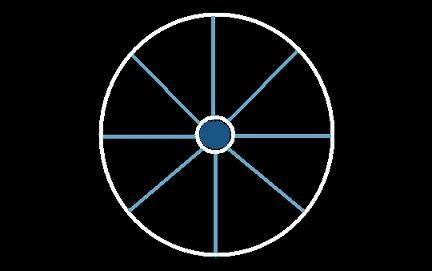
The previous section Part I introduced the Octagon A algorithm for the construction of 5×5 Wheel Squares. This section will cover the 7th order squares which unlike the 5th order has many more non spoke white cells which require three Octagon A methods independent of each other. The square will be built according to Part I starting with the initial node at top left.
In Part I the Number of Squares (NS) for a 5×5 square was listed as three. To determine NS for higher order n it was found that n was related to a variable d which was the term number of the Sloane sequence A002378 stored in the OEIS database:
for d ≥ 0 and where each term in the Sloane sequence was found to be one less than the Number of Squares. This led to the series of equations (a) thru (d) giving NS based solely on the order n.
| d = (n − 3)/2 | (a) | |
| d(d + 1) = (n − 3)/2 [(n − 3)/2 + 1] | (b) | |
| d(d + 1) = (n2 − 4n + 3)/4 | (c) | |
| NS = d(d + 1) + 1 = (n2 − 4n + 7)/4 | (d) |
In addition, while (d) was found useful for calculating NS, the sequence containing the NS terms were also to be found in the OEIS database under the Sloane number A002061, thus, confirming my approach. Moreover, taking (d) and plugging in the values 5 and 7 afforded 3 and 7, respectively, while plugging in the value of 3 for a 3×3 square, afforded NS=1, the value consistent for a single square.
The following table shows the first 24 numbers from a 7×7 complement table not including the central number of the square and the complements since shifting these 24 numbers also shifts their complements an equal amount. The wheel spoke numbers have been shifted to the right every two cells to avoid leaving behind unpaired complementary pairs. Thus, the number of squares that can be constructed using this particular algorithm is indeed 7 as confirmed by (d).
| 0 | 1 | 2 | 3 | 4 | 5 | 6 | 7 | 8 | 9 | 10 | 11 | 12 | 13 | 14 | 15 | 16 | 17 | 18 | 19 | 20 | 21 | 22 | 23 | 24 | |
|---|---|---|---|---|---|---|---|---|---|---|---|---|---|---|---|---|---|---|---|---|---|---|---|---|---|
| 1 | 1 | 2 | 3 | 4 | 5 | 6 | 7 | 8 | 9 | 10 | 11 | 12 | 13 | 14 | 15 | 16 | 17 | 18 | 19 | 20 | 21 | 22 | 23 | 24 | |
| 2 | 1 | 2 | 3 | 4 | 5 | 6 | 7 | 8 | 9 | 10 | 11 | 12 | 13 | 14 | 15 | 16 | 17 | 18 | 19 | 20 | 21 | 22 | 23 | 24 | |
| 3 | 1 | 2 | 3 | 4 | 5 | 6 | 7 | 8 | 9 | 10 | 11 | 12 | 13 | 14 | 15 | 16 | 17 | 18 | 19 | 20 | 21 | 22 | 23 | 24 | |
| 4 | 1 | 2 | 3 | 4 | 5 | 6 | 7 | 8 | 9 | 10 | 11 | 12 | 13 | 14 | 15 | 16 | 17 | 18 | 19 | 20 | 21 | 22 | 23 | 24 | |
| 5 | 1 | 2 | 3 | 4 | 5 | 6 | 7 | 8 | 9 | 10 | 11 | 12 | 13 | 14 | 15 | 16 | 17 | 18 | 19 | 20 | 21 | 22 | 23 | 24 | |
| 6 | 1 | 2 | 3 | 4 | 5 | 6 | 7 | 8 | 9 | 10 | 11 | 12 | 13 | 14 | 15 | 16 | 17 | 18 | 19 | 20 | 21 | 22 | 23 | 24 |
For instance, the first line of this table can be used to construct Magic Square 7(0), where (0) signifies no shift, otherwise the number of shifts increase by two as one goes down the table. The first column in bold is a number also used in the coded programs (the variable knum) to access the correct wheel structure (the cells in brown). First the Wheel 7(0) partial square is constructed using the Wheel algorithm Part I then followed up using the directed graph Octagon A algorithm. Since Wheel 7(0) has 24 empty white cells, we require three Octagon A methods of eight numbers apiece to complete the square each starting at a node 1. Therefore, 10, 14 and 18 each belong to a different node 1 each followed by three consecutive numbers and four consecutive complements, placed in their appropriate cells and equidistant from the center cell. To wit: three sets of four consecutive numbers (10,11,12,13), (14,15,16,17) and (18,19,20,21) followed by three sets of their complements, where a number and its complement sum to 50.
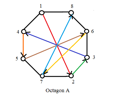
In addition, there are included the sums of each row, each column and the left diagonal for both the partial wheel and the magic square after construction of the wheel and upon completion of the square. To distinguish the internal Octagon from both of the external Octagon ones, the four numbers beginning with 18 and their complements are pictured in light blue. Computer coded examples of the 7×7 squares will be shown at the end of this page.
|
⇒ |
|
As stated above, whenever the wheel construct produces a lone complement pair the result is a non magic square where (s1) signifies a shift of one to the right in the complement table (not included in Table I above):
|
⇒ |
|
The result being that one row and one column are less than the magic Sum of 175, thus confirming that adjacent pairs must be kept together.
Coding for these involves first constructing the wheel using the Wheel algorithm. The coding part using the Octagon A algorithm for the 7×7 may be done in either of two ways. The first is to access the numbers left over after the wheel spoke numbers have been removed from the array, viz., numbers 10 to 40. The program retrieves the numbers in three groups of four until each number has been removed. Then it retrieves the complements, also in three groups of four until the array is empty. This method attempted to follow the original 5×5 method of Part I but had to be modified because of the way the numbers are retrieved from the array (from left to right consecutively).
Thus for the zero number square in Table I where all the Wheel spoke numbers have been deleted, the array is initially:
After the first 12 numbers are retrieved and removed from the array, the array stands at:
In the second method the first four numbers are consecutively retrieved, deleted from the array and followed by a search for the four complements of these numbers. Once found the complements are retrieved and deleted from the array leaving the array at:
Both methods eventually remove every number from the array until only zeros remain in the array. The former method can be considered to be a modified Octagon algorithm because of the way the search and retrieval of numbers are performed. The latter method, however, follows the true algorithm employed by someone using paper and pencil even though both methods happen to produce the same identical magic squares.
In addition, the code for the programs also update the sums of all the rows and columns each time a number is entered into the square. Below are six programs for both methods described above where the first three numbers in column one of Table I, (viz., knum=0,1,2 values in the coded programs) are used to generate the series of squares. First the wheel is filled in, then, the Octagon algorithm takes over to fill the square step by step, one number at a time until the square is filled and the array is empty except for zeros.
| (a) Octagon Aa0 and text file Octagonal A-1 text |
| (b) Octagon Aa1 |
| (c) Octagon Aa2 |
| (d) Octagon Ab0 and text file Octagonal A-2 text |
| (e) Octagon Ab1 |
| (f) Octagon Ab2 |
Go back to Part I. Go to Part III 9×9 Squares. Go back to homepage.
Copyright © 2022 by Eddie N Gutierrez. E-Mail: enaguti1949@gmail.com