Octagon Algorithm for Wheel Magic Squares (Part I)

A Synopsis of Previous Work

In the past odd nth order magic squares have been constructed via a number of different algorithms, for example, the most commonly known is the Loubère staircase method. A different type of odd magic squares is based on what I call the Wheel Algorithm, a completely new type of construction, as shown in variant1 and variant27 from 2008. However, at that time the squares were depicted with the main diagonal as the left diagonal. This has been corrected to the way we are accustomed to seeing this square: the right diagonal is the main diagonal just like in the Loubère case. In addition, the initial number is placed in the central top cell also like in the Loubère case, whatever that initial number may be which in this case is Wheel A:

and uses the accompaning 5×5 complementary table as a guide to pick the 17 wheel spoke numbers:

Depicted in this manner it can be seen that:

where all the numbers and their complements were extracted from the complementary table, leaving eight non spoke numbers for completing the square, and where the main diagonal is obtained from ½(n²-n+2) to ½(n²+n).

It was also shown in Variant1 that the 5×5 complementary table has two other conformations, viz.:

where the non spoke numbers in white cells must be present as pairs of complementary numbers since a single unpaired complement will lead to non magic squares. For example, on the left complement table, (1,25) and (2,24) must be both in white. If (1,25) is white and (2,24) is brown this leaves (1,25) alone and unpaired. In addition, as the spoke numbers in brown move to the right of the complement table, the topmost central numbers are 3 and 5, respectively.

It was shown previously that after the construction of the wheel the non spoke numbers were filled in according to parity which requires calculations to be performed on the rows and columns, a very tedious affair. Those results, although they show what sums (odd/even parity) are necessary to fill in the column and rows, need not concern us here. I have found that an algorithm employing graph theory (just follow the arrows) is all that is required to fill in the rest of the numbers. It works for any size odd square and works best using pencil, paper and a good set of eyes.

One caveat, however, the algorithm can be transcribed into computer code but works best for small nth order squares. The bigger the n the more section of coding required just for the non spoke section. For example, eight sections are needed just for the 5×5 square which increases to 24 for n=7 and 48 for n=9. The problem here is that we can't use for or while loops as was used for coding the Staircase Squares where the coordinates, (row,column), for moving up the stairs are constant numbers. Here each section requires a different coordinate, (row,column). (See Computer Coding section at the end, specifically the text version). More of this in Part II.

The Octagonal Algorithm-The Eight Node Way

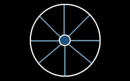
If one looks above at Square Wheel A one notices that the 8 white cells are arranged as the vertices or nodes of an octagon. I found that the non spoke numbers can be filled in by employing an octagon and its nodes as part of the algorithm and adding directed edges (arrows), in color, to form a directed graph. The direction of the arrows tells me to start at node 1, then node 2 ... and finish at node 8, placing a number from the complementary table at each node (white cell). For instance, any node may be number one, but for the sake of argument I will consider node one in either of the two positions shown below.

Nodes 1-4 are filled in with the top four numbers from the complementary table, while 5-8 are filled with the bottom four, i.e., the complements of nodes 1-4. Or nodes 1-4 are filled in with the bottom four numbers from the complementary table, while 5-8 are filled with the top four while ensuring that the non spoke numbers are inserted into the square in the correct order. The result, in any event, is that magic squares are produced having slightly different configurations. It can be seen that the adjacent nodes (1,8), (2,7), (4,5) and (3,6) each sum to 9 and any deviation from this value results in improper values being placed into a cell of the square. In other words, these are the only four tuples allowed. In addition, a certain number of edges must intersect thru the center.

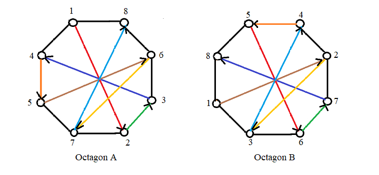
Note that we have two directed graphs, A and B, both with four intersecting edges, two edges which are part of the octagon and one non intersecting edge which is not part of the octagon (very similar looking to a wheel). And where the intersection of edges is the number 13 on the square. Therefore, employing Octagon A algorithm on Wheel A yields Magic Square A, while using the Octagon B algorithm yields Magic Square B:

From these two squares it may be seen that the complementary nodes (1,8), (2,7), (4,5) and (3,6) do indeed produce complementary values in the square whose sum is 26. And it doesn't end here. Octagon C with node 1 in the same position as Octagon B can take a route different from the other two, while Octagon D is similar to A but with (3,6) and (4,5) reversed:

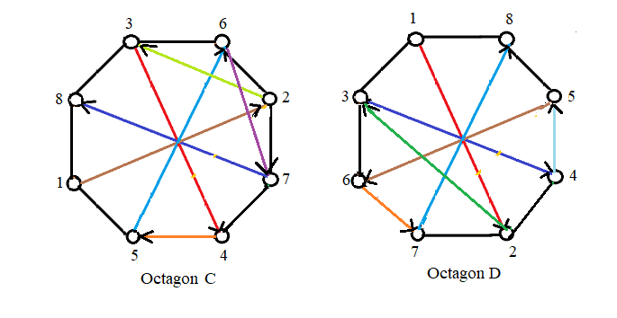
yield Magic Squares C and D:

Note that this square may also be constructed from Octagon A if the first number 9 is considered to be node 1. The numbers that follow 9 are, however, partially consecutive and seem to follow a route that is somewhat circuitous.

Computer Coding for 5×5 Square

Although three Octagonal algorithms have been depicted, I will concentrate all my efforts on Octagon A, to keep things simple. The 5×5 has been coded into three programs below using the three complementary tables at the beginning of this page along with one text file showing the coding itself. These programs first fill the wheel part in one step, then proceed to use the Octagon A method step by step. In the programs, the squares are depicted with sums of rows (last column), sums of columns (last row) and sum of the left diagonal. After construction of the wheel portion the sums of all row and columns along with the left diagonal are set to their initial values which change after each insertion of a number into a cell. In addition, there is an array of numbers bearing only the non spoke numbers (the spokes have been deleted from the list). A number from the array is removed after its insertion into a cell and the next number on the list is obtained by moving to the right of the array until the list contains zeros. The first program generates Magic Square A, while the second and third give squares where the spoke numbers are shifted by two and four numbers, respectively .

This completes the Octagon A method. Go to 7×7 Squares. Go back to homepage.